~
Increasingly individuals from the United States are aware of the value of health insurance. The percent of individuals without health insurance has been steadily falling from 18% in 2013 to nearly 11% in the beginning of 2015. Before we can even begin to discuss policy, we need to understand the people at risk. Who doesn’t have insurance? How difficult is it to get it to them? What is the problem?
These questions could be purely political or philosophical questions. Or we could turn our eyes toward more rigorous investigation. Using the American Community Survey (ACS), we have access an enormous array of information about millions of Americans. There are over 280 different questions asked. Of these, one is whether the person has health insurance. Instead of asking simple questions about what percentage have insurance, let’s ask what do the other questions tell us about these individuals. I used 2012 data, but the results and investigation are robust to any survey.
Through the use of python’s scikit-learn supervised learning packages we can try to create models to predict whether or not an individual has health insurance. What this means is that it will use the content of all of the other questions answered to find whether this individual is likely to have insurance. Potentially we can find out what about their responses give us hints about potential structural challenges in their lives.
In summary, I aimed to create a model that can accurately predict whether an individual has acquired health insurance, as well as identify the top factors involved in an accurate prediction. I used psycopg2 to input the data into a Postgresql database, and multiple scikit-learn supervised learning algorithms to investigate this question.
Squeezing The American Community Survey Data For All It’s Got
Before doing any AMAZING data science, we first have to figure out how we are going to handle the enormous amount of data that the American Community Survey has to give. Here in lies the problem: 284 columns, and over 3 million individuals. Each of these columns are non-obvious. Some involve the number of cars you own. Some talk about the employment category. Some talk about the number of bathrooms in the house. Clearly some are more interesting than others. Knowing the exact hour that an individual goes to work may not help us to our goal. Knowing whether or not they have social security support may be extremely relevant. So before doing anything I had to comb through the hundreds of questions to identify their viability.
But wait! There is a problem. After looking through all the columns, it is clear we have an issue. Only 12 of over 284 columns are numerical. All of the others are categorical. What problem does this pose? Machine learning algorithms treat all numbers as magnitude. In one of the employment columns, we have employment codes that could have the value 3900. Is this a really large job? Unfortunately that is how a supervised learning algorithm would see it. So we need to create something called Dummy Variables. This is where each employment code would get its own column. The value of this column can be either 1 or 0. It either is or isn’t that job. All the categorical columns have this issues. Another example is ethnicity: They either are or are not from the Pacific Islands. (the last sentence was random, you only talked about jobs in this paragraph, not ethnicity)
Herein lies the problem. If the race column has over 200 categories, that means over 200 new columns added to the data. Nearly all of the questions are categorical and dozens have a large number of coded answer choices. The curse of dimensionality is something to be careful about when dealing with a ballooning number of features.
To move forward I removed the majority of columns on two points: relevance to health insurance, and number of features added to our data. This left me with a little over 70 columns and ~1000 features. Given the enormity of the data set the 1000 features shouldn’t be too large a task. It is a large improvement over the 10,000 features that would be created from an unfiltered dataset.
I use the python pandas model to handle all of my data needs. This includes using the get_dummies module to create dummy variables from categorical variables.
In addition, I filtered the data by age greater than 18, scaled the numerical data, and dropped columns with too many N/A results.
Databasing
Once we have our nice and tidy dataset we can move toward databasing. I chose to database this dataset for later extraction and sql based interaction. I chose to use Postgresql database.
I read the data into pandas by chunk. I created the table if it wasn’t already present, and dynamically created columns if they weren’t previously there. Because of the large number of N/A responses by individuals - and the large number of features - some features may not be seen until later chunks. Dynamically adding columns and inserting values is non-trivial in SQL.
Here is how I handle dynamic INSERT statements:
sql = "INSERT INTO test (%s)" % ','.join("%s" % col for col in chunk.columns)

sql = sql + " VALUES (%s);" % ','.join('%s' % col for col in chunk.iloc[i])
Modeling and Results
I created 4 models for the prediction: Naive Bayes, Decision Trees, Logistic Regression, and Random Forest. All of these are from the sic-kit learn python modules.
I then ran learning-curves the first three using over 200,000 points.
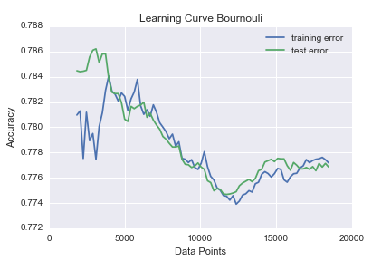
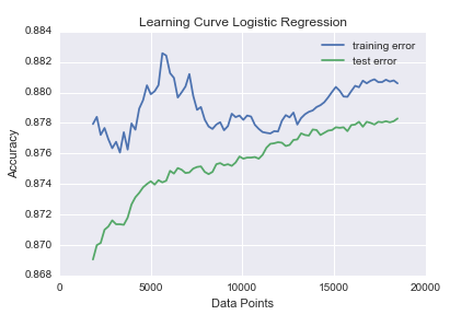
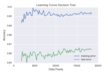
There is quite erratic behavior for both the Naive Bayes and Logistic regression. I believe this is because of the readjustments for new columns added as new data comes in. The Decision tree starts converging around 5000 data points, which is a small fraction of our data. This is a successful result because I was intending to focus on Random Forests as a model. A Random Forest is an ensemble of randomly generated Decision Trees.
Accuracy scores of the models including a Random Forest Classifier:
| Naive Bayes |
|---|
| 0.78 |
| Logistic Regression |
| 0.879 |
| Decision Trees |
| 0.865 |
| Random Forests |
| 0.88 |
These are all fairly good results. The percent of people who had insurance during the year of 2012 was ~82%. This a ~7% gain over a completely overfit solution.
The advantage in using a Random Forest is that we can pull out the top features that are associated with accuracy.
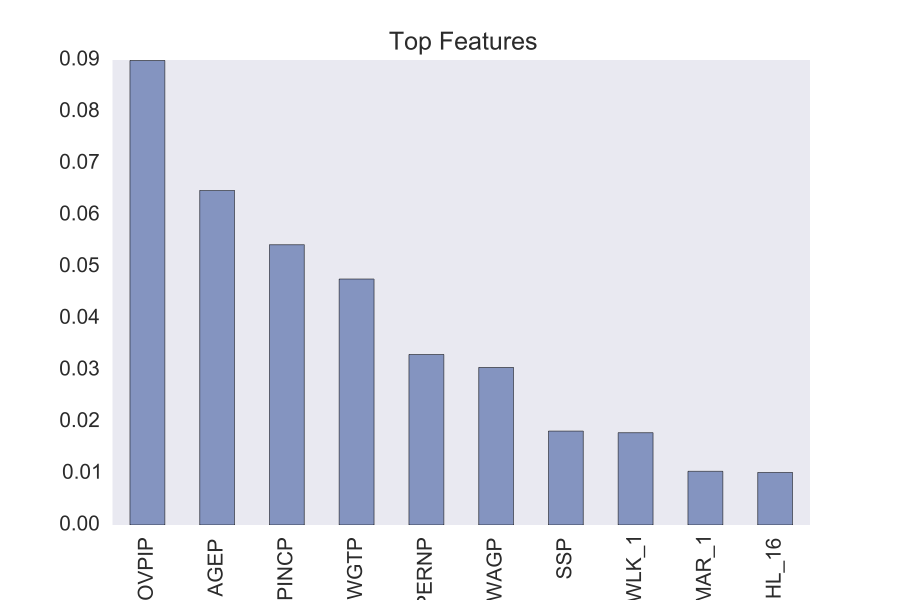
The first feature is the poverty-income ration. This is a key measure of poverty in the United States. The next obvious ones are age and income. It also appears that the individuals weight is a fairly good indicator of health insurance coverage.
These results are great in that they make sense and support the idea that our model functioned appropriately. Beyond this we have a challenge of investigating how these features affect our results. The unfortunate quality of getting top features from a Random Forest is that you don’t know which direction they influence. Does being poor or rich associate with having insurance? Maybe it is that the wealthier people can afford the insurance. Maybe the poorer have Medicare. Features like weight are especially interesting. How does the individuals weight affect health care coverage? More interestingly is why? We all can guess. But now we have some results to start guessing over.
Take-Away
Through the use of supervised learning algorithms, there is support that we can identify people at risk of being without health insurance. What is possibly more interesting is that we can look at the individuals who were misclassified as having insurance. These people may be a part of an underserved group.
The power of investigating population data with machine learning tools can not be overstated. The American Community Survey was created to find the best way to distribute resources from the government. We should use every method at our disposal.
View complete code at https://github.com/agatorano/Census_Insurance_Prediction
2016: Andre Gatorano